3. Interface and Function Description
3.1. Online Tuning Interface and Function Description
3.1.1. Tuning Structure Interface
After opening the CviPQ tool for online operation, the tuning table panel on the left side of the tool displays the tunable items of all modules. The structure is shown in Fig. 3.1.
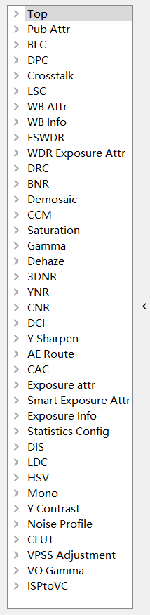
Fig. 3.1 The structure of the left side of the tool
Click the tunable items of these modules, and the corresponding tuning page of the module will be displayed in the tuning area on the right side of the tool, providing users with adjustment parameters, as shown in Fig. 3.2.
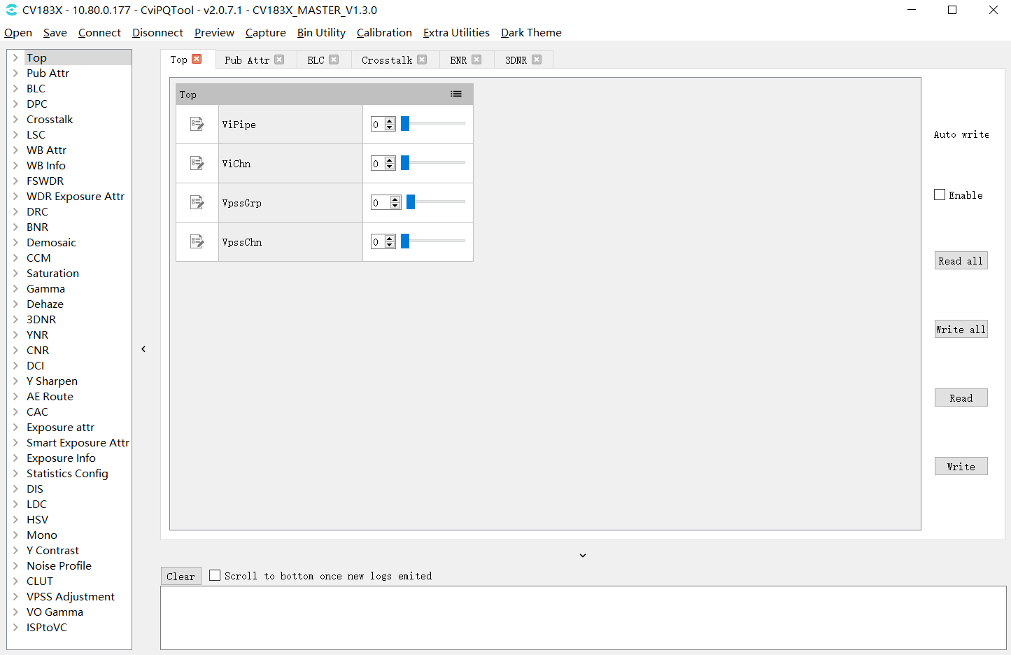
Fig. 3.2 Tuning page
3.1.2. Register / Algorithm Parameter Adjustment
Each item in the list on the left side of the tool interface is the “register / algorithm parameters” tuning page. The tuning interface corresponding to these pages is shown in Fig. 3.3. All parameters in the debugging page corresponding to each module will be divided into several groups according to different functions.
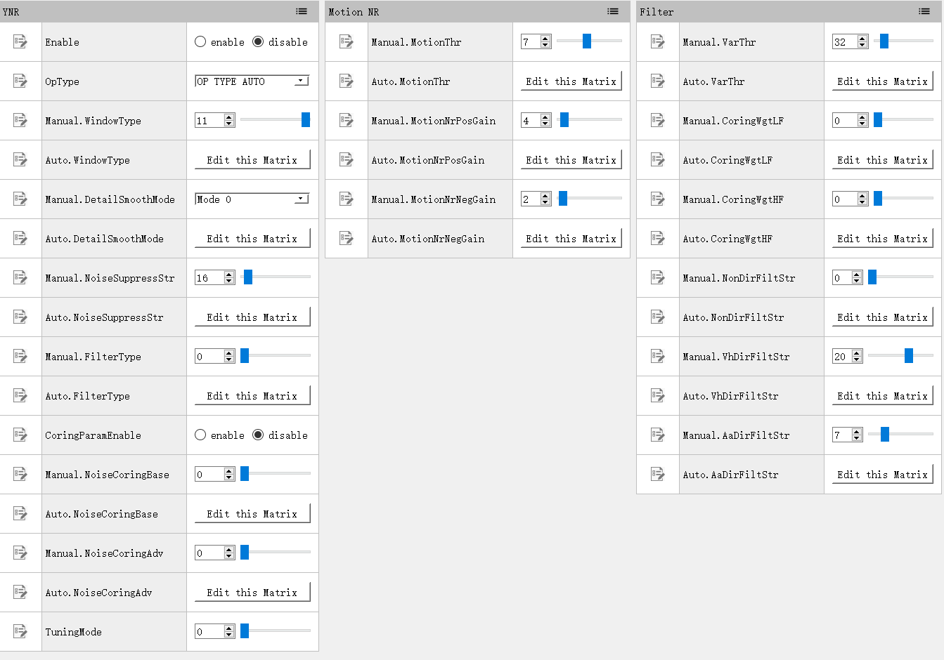
Fig. 3.3 Tuning page of register / algorithm parameters (take YNR as an example)
3.1.2.1. View and Modify Register / Algorithm Parameters
Each group contains registers and algorithm parameters, in which the parameters marked with “  ”are read-write and the parameters marked
with “
”are read-write and the parameters marked
with “  ”are read-only.
Parameters are divided into the following categories according to their properties and value ranges, which are presented in different forms of
controls, as shown in Table 3.1 .
”are read-only.
Parameters are divided into the following categories according to their properties and value ranges, which are presented in different forms of
controls, as shown in Table 3.1 .
Type |
Description |
Control Operation |
|---|---|---|
Boole |
either-or |
Set and view through the check box: 
|
Neumerical Value |
Real number with a certain range of values |
Use the following controls to adjust and view values: 
The values can be adjusted in the following wa 1.Enter the value directly in the text box 2.Click the small arrow on the right side of the text box to fine tune up and down 3.Drag the right slider |
Enumeration |
Multiple choice |
Set and view values through the drop-down box: 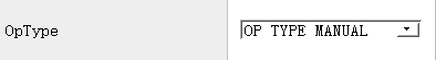
|
Matrix |
Multibyte Sequence |
The tuning page will display a button to edit the matrix. If the matrix is read-only, the button to view the matrix will be displayed. 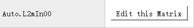
Click the button to open a dialog box, in which the corresponding matrix values are displayed in the form of a table. The user can modify the values in the table. If the matrix is read-only, it can only be viewed. Users can click Import / Export to import and export matrix values, and only the “Export” button is available for read-only matrix. 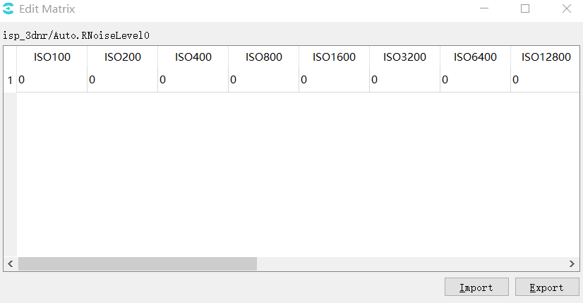
|
3.1.2.2. Read Data from Board End
When the tool is connected to the board end, click the read button( )on the rightmost side of each module page.
The tool will read the value of each parameter on the current board and update it to the interface.
)on the rightmost side of each module page.
The tool will read the value of each parameter on the current board and update it to the interface.
3.1.2.3. Write Parameters to the Board End
When the tool has been connected to the board, click the write button( ),on the far right of each module page, and the tool will write each
writable parameter on the module page to the board.
),on the far right of each module page, and the tool will write each
writable parameter on the module page to the board.
3.1.2.4. Parameter Temporary Storage and Recovery
The tool provides four groups of data temporary storage space for each tuning group. The user can use the “To Set” button to save the adjusted values of parameters, and then use the “Load Set” button to restore and compare. The detailed operation instructions are shown in Fig. 3.4 . Please refer to the following instructions.
When this icon is selected, the quick buttons of parameter temporary storage and recovery can be displayed
Click the “To Set” button to save the current parameters temporarily. Different values can be stored in different Sets temporarily for quick recovery later.
Click the “Load Set” button to restore the previously stored value. Take Fig. 3.4 as an example: If the user has stored “Set1” and “Set2” two groups of values temporarily, “Load Set1” or “Load set2” button can be used to quickly recover and compare them.
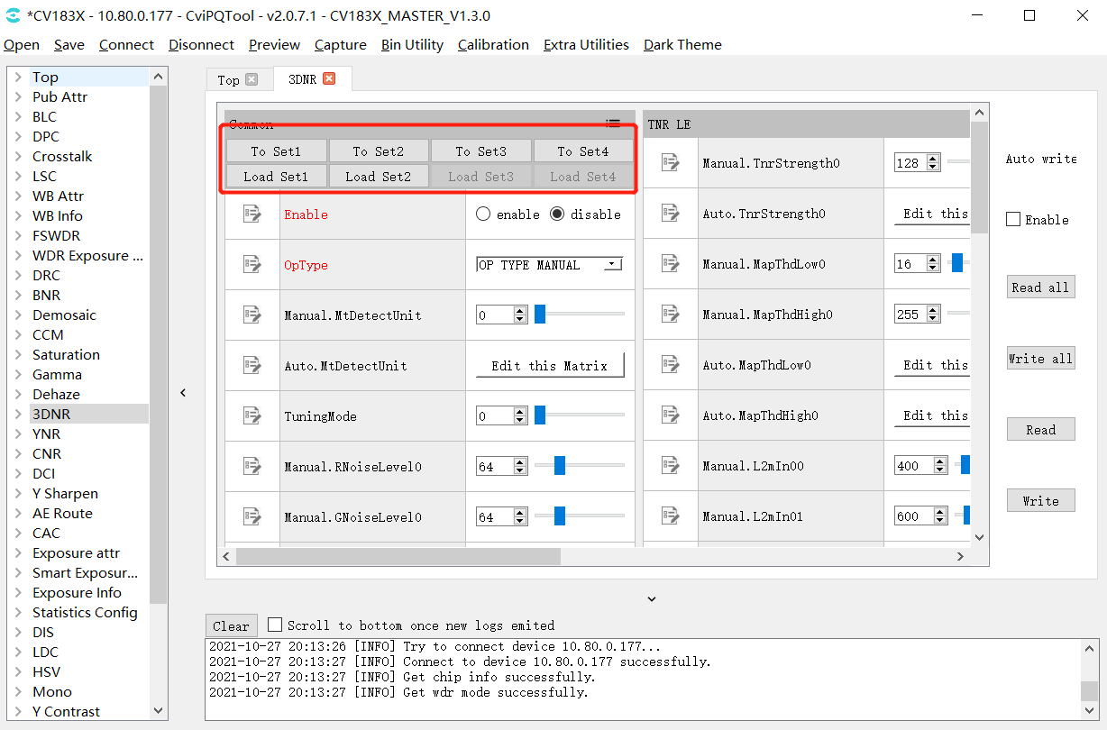
Fig. 3.4 Parameter temporary storage operation interface (taking 3DNR as an example)
3.1.3. Batch Reading and Writing and Automatic Writing of Tuning Data
When open the tuning tool and enter the main interface, you can see the data read / write control interface on the far right, as shown in Fig. 3.5.

Fig. 3.5 Data read / write control interface
To operate the read / write console, you need to connect the tool to the board first, with the following specific functions:
Read All Button:When this button is clicked, the tool will read the current value of all module page parameter items on the board. It is suggested that before opening the tool for tuning or after importing the Bin file, all read operations should be performed once.
Write All Button:When this button is clicked, the tool will write the values of all module page parameter items to the board.
Auto Write Switch:When this option is checked, the tool will write the new value of the parameter to the board each time a writable parameter item is adjusted. It is recommended to open this item during tuning to ensure that the adjustment value can take effect immediately.
Write Button:When this button is clicked, the tool will write the values of all parameter items in the currently opened module page to the board end.
3.1.4. Curve Visualized Tuning
3.1.4.1. General Curve Function Description
The generic curve in the tool is shown in Fig. 3.6. For example, in the 3DNR debug page, click the Edit this Curve button to enter the curve window.
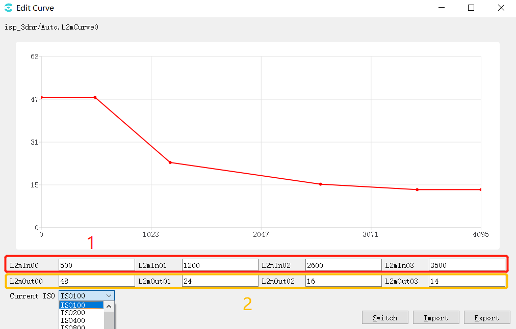
Fig. 3.6 3DNR page curve operation example diagram
In the figure, 1 is the horizontal coordinate of the curve, 2 is the vertical coordinate of the curve, corresponding to the 4 points in the curve, modify their values, and the points on the curve will change accordingly; you can also drag the points on the curve by the mouse, corresponding to the horizontal and vertical coordinate values change with it.
Current ISO: drop-down option to select different ISO values and view their corresponding curves.
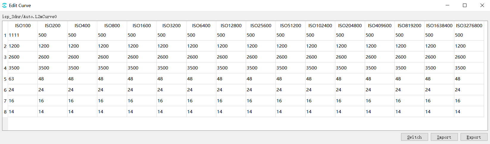
Switch: mode switch button, click in curve mode, enter the following table mode, the first 4 lines of the table are horizontal coordinate values, the last 4 lines are vertical coordinate values, the table can be edited.
Import:import parameters from the file.
Export:export parameters to the file.
3.1.4.2. Gamma Visual Tuning
Click Gamma page on the left list of tuning tools to enter Gamma visual tuning page, as shown in Fig. 3.7.
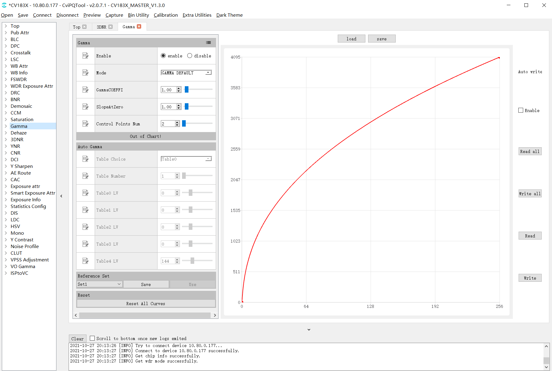
Fig. 3.7 Gamma Tuning Page
The following is the specific parameter description and usage:
Gamma
Enable parameter, set it to enable Gamma.
Mode parameter, represents the curve adjustment mode, when GAMMA_DEFAULT/GAMMA_sRGB is chosen, the curve will be reset to the default curve, and the user can’t adjust the curve manually. When GAMMA_USER_DEFINE is chosen, the the curve will be reset to a straight line with the starting point of (0,0) and the ending point of the maximum value of X / Y axis. The user can manually adjust the direction of the curve.
GammaCOEFFI parameter, restore the current curve to a standard gamma curve (coefficient range 0.01 to 20.0) by entering a value in the text box or dragging the slider.
SlopeAtZero parameter, adjust the slope of gamma curve at zero point (the slope range is 0.01 to 20.0) by inputting a value in the text box or dragging the slider.
Control Points Num, When GAMMA_USER_DEFINE/GAMMA_AUTO is selected, by adjusting this parameter, the user can set the number of control points that can be operated.
Auto Gamma (gamma mode set to GAMMA_AUTO is valid )
Table Choice , select gamma table 0 ~ 5 according to light value, currently using the first 4 groups.
Table Number, number of tables currently in use.
Table0~4 LV, corresponds to 5 light value valves (LV:-5~15).
Reference Set
Curve data temporary storage area, the tool provides three sets of temporary storage space from set1 to set3, the user clicks the save button the current curve data will be saved to the selected set, and the user clicks the use button the temporary stored data can be restored to the curve interface. By default, the use button is grayed out and unclickable when no temporary storage operation is performed.
Reset
Reset is the reset button. After clicking, the curve will be reset to a straight line with the starting point of (0,0) and the ending point of the maximum value of X / Y axis.
Load&Sav
Click the “Load” button to read the curve data from the file, write it back to the tool data cache, and refresh the display curve at the same time.
Click the “Save” button to save the current curve data to the local text file. The tool supports two formats of data files:Cvitek Json file and Other text file
Click the “Read” button of the page read / write control interface, the tool will read the curve data from the board end and refresh the curve display.
Click the “Write button”, and the tool will write the data of the current curve to the board end.
If “Auto Write” is checked, when the curve is adjusted, the data of the curve will be automatically written to the board end to take effect.
3.1.4.3. VO Gamma
Click VO Gamma in the left list of tuning tool to enter the VO Gamma visual tuning page, as shown in Fig. 3.8.
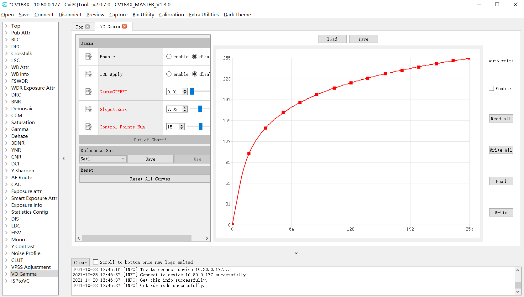
Fig. 3.8 VO Gamma tuning page
Parameters description:
Gamma
Enable, set it to enable VO Gamma
OSD Apply, display watermark switch.
GammaCOEFFI parameter, restore the current curve to a standard gamma curve (coefficient range 0.01 to 20.0) by entering a value in the text box or dragging the slider.
SlopeAtZero parameter, adjust the slope of gamma curve at zero point (the slope range is 0.01 to 20.0) by inputting a value in the text box or dragging the slider.
Control Points Num, when GAMMA_USER_DEFINE/GAMMA_AUTO is selected, by adjusting this parameter, the user can set the number of control points that can be operated.
Reference Set
Curve data temporary storage area, the tool provides three sets of temporary storage space from set1 to set3, the user clicks the save button the current curve data will be saved to the selected set, and the user clicks the use button the temporary stored data can be restored to the curve interface. By default, the use button is grayed out and unclickable when no temporary storage operation is performed.
Reset
Reset is the reset button. After clicking, the curve will be reset to a straight line with the starting point of (0,0) and the ending point of the maximum value of X / Y axis.
Load&Sav
Click the “Load” button to read the curve data from the file, write it back to the tool data cache, and refresh the display curve at the same time.
Click the “Save” button to save the current curve data to the local text file. The tool supports two formats of data files:Cvitek Json file and Other text file
Click the “Read” button of the page read / write control interface, the tool will read the curve data from the board end and refresh the curve display.
Click the “Write button”, and the tool will write the data of the current curve to the board end.
If “Auto Write” is checked, when the curve is adjusted, the data of the curve will be automatically written to the board end to take effect.
Usage:
Tool is connected to the board end normally, and the board end is connected to the display to output images normally.
Use the “GammaCOEFFI”, “SlopeAtZero”, “Control Points Num” functions to adjust a desired curve.
Select enable for “Enable” and click write.
Observe the display and the image brightness will change.
3.1.5. Exposure Data Status and Parameter Setting
3.1.5.1. Exposure Data Status
The Exposure Info page can display the current exposure data status, including exposure time, gain, ISO, etc. As shown in Fig. 3.9.
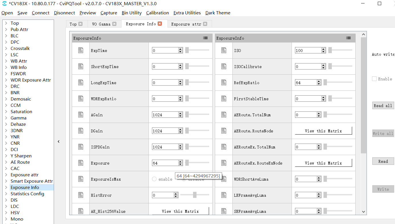
Fig. 3.9 Exposure data status page
3.1.5.2. Exposure Parameter Setting
The Exposusre Attr page can set the exposure related parameters, including exposure time, gain, ISO, etc. As shown in Fig. 3.10.
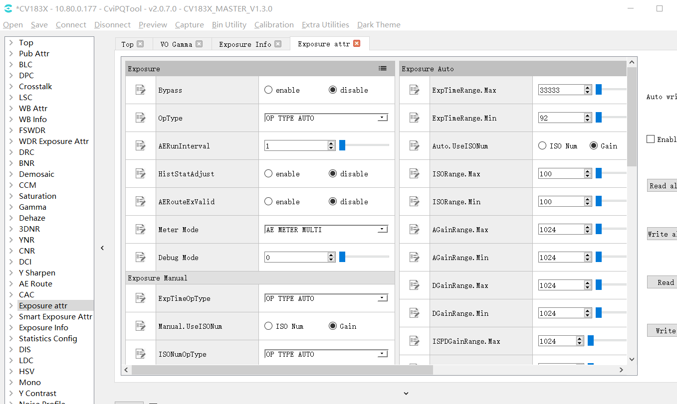
Fig. 3.10 Exposure parameter setting page
3.1.6. White Balance Data Status and Parameter Setting
3.1.6.1. White Balance Data Status
WB info page can display the current white balance data status, including gain, color temperature, etc. As shown in Fig. 3.11.
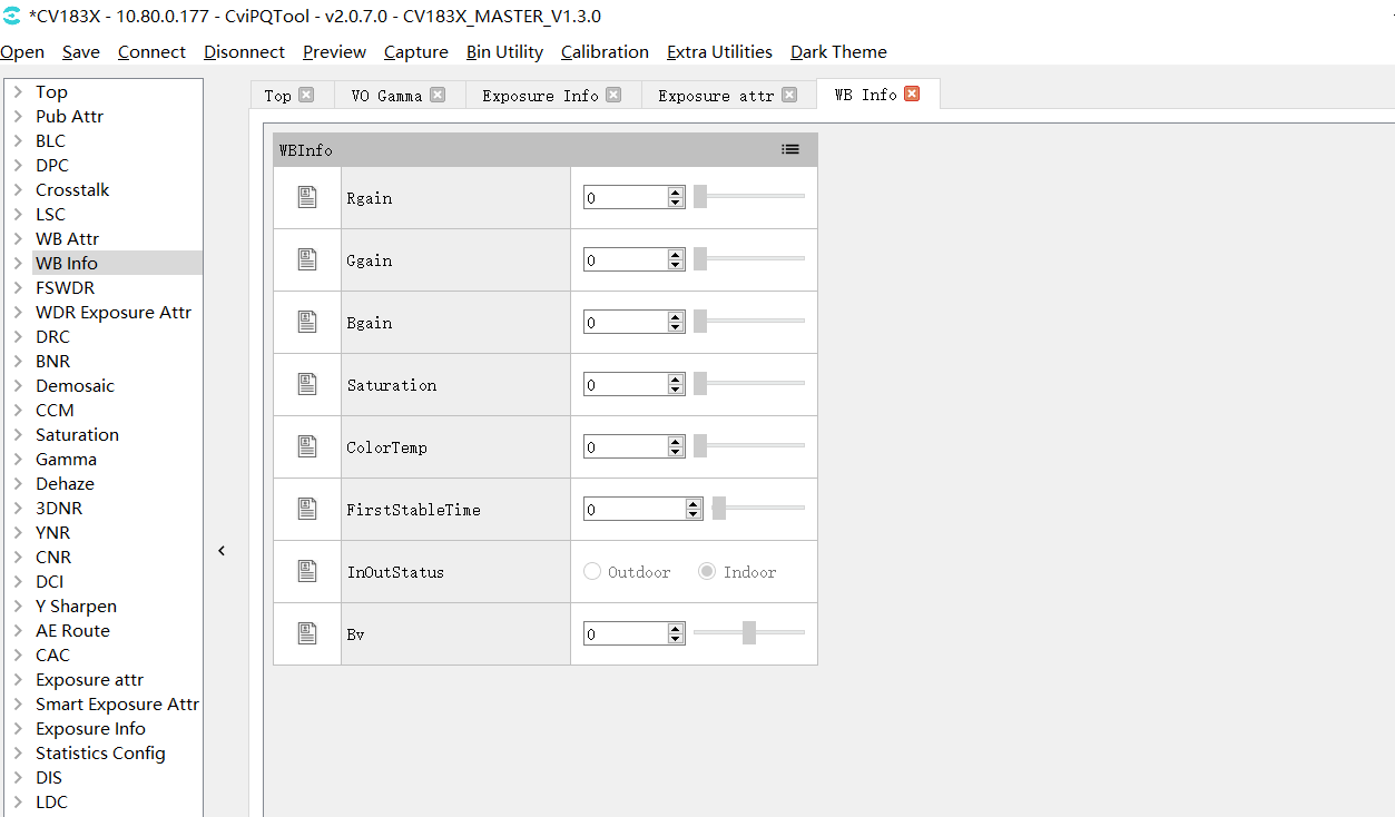
Fig. 3.11 White balance data status page
3.1.6.2. White Balance Parameter Setting
WB attr page can be set white balance related parameters, including gain, color temperature, etc. As shown in Fig. 3.12.
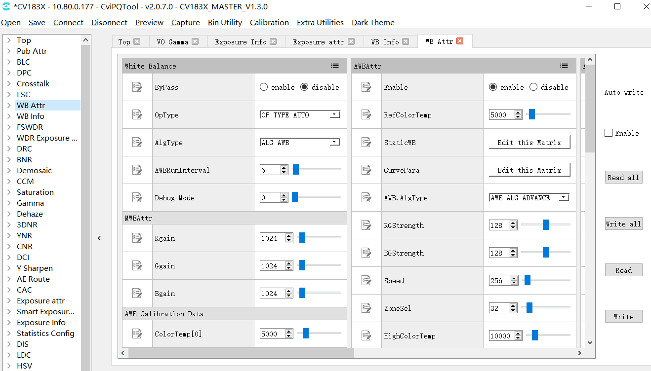
Fig. 3.12 White balance parameter setting page
3.1.7. WDR Exposure Parameter Setting and Local-Tone Switch
For detailed description of WDR and DRC parameters, please refer to section WDR and section DRC from “ISP Tuning Guide”.
3.1.7.1. WDR Exposure Parameter Setting
WDR Exposusre Attr page can be set wide dynamic exposure related parameters, including exposure ratio, etc. As shown in Fig. 3.13.
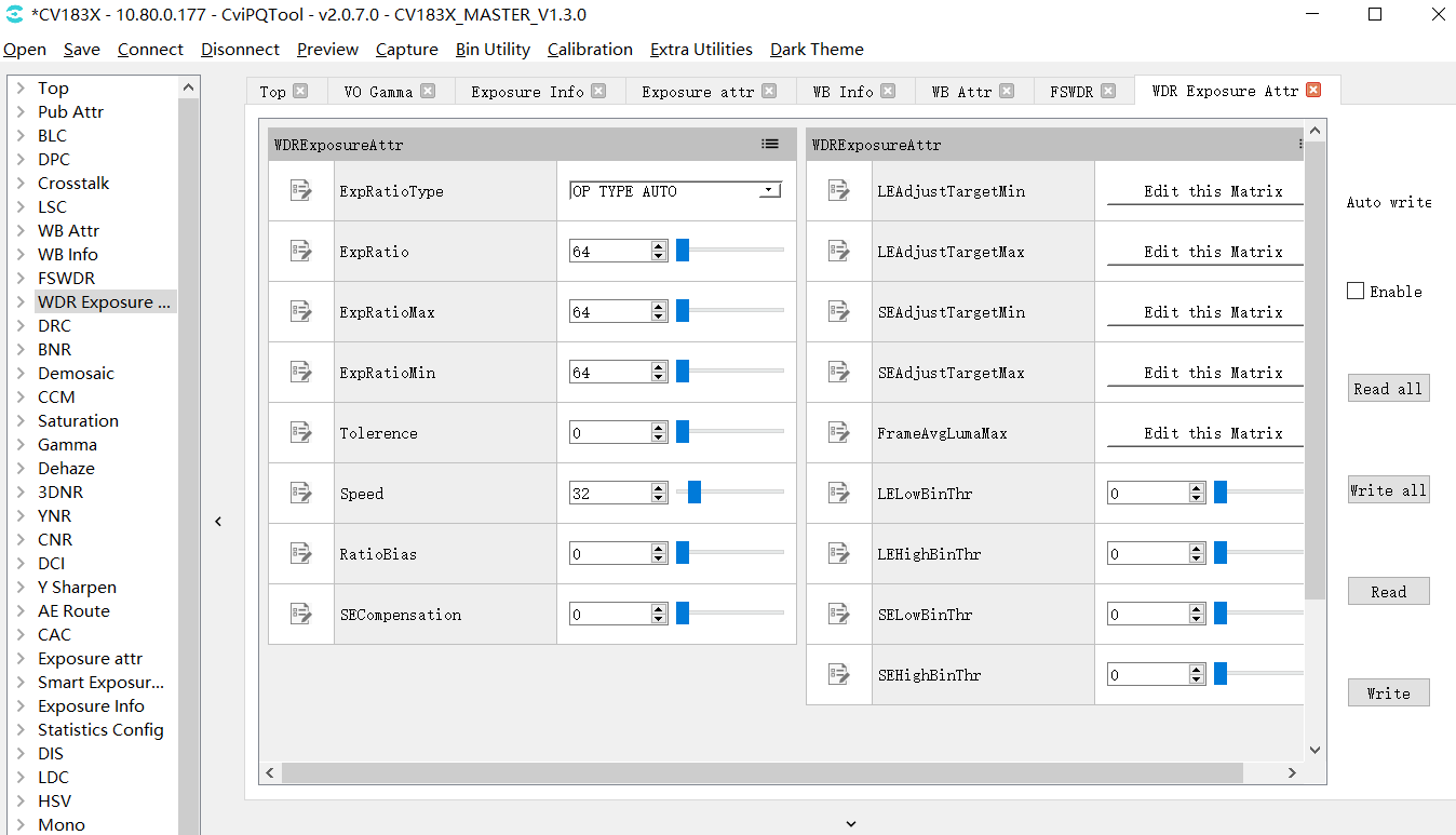
Fig. 3.13 WDR exposure parameter setting page
3.1.7.2. Local-tone Switch
Local-tone can be turned on or off on the DRC page. When the [LocalToneEn] parameter is set to enable, it means that the Local-tone is turned on. When the [LocalToneEn] parameter is set to disable, it means that the Local-tone is turned off, as shown in Fig. 3.14.
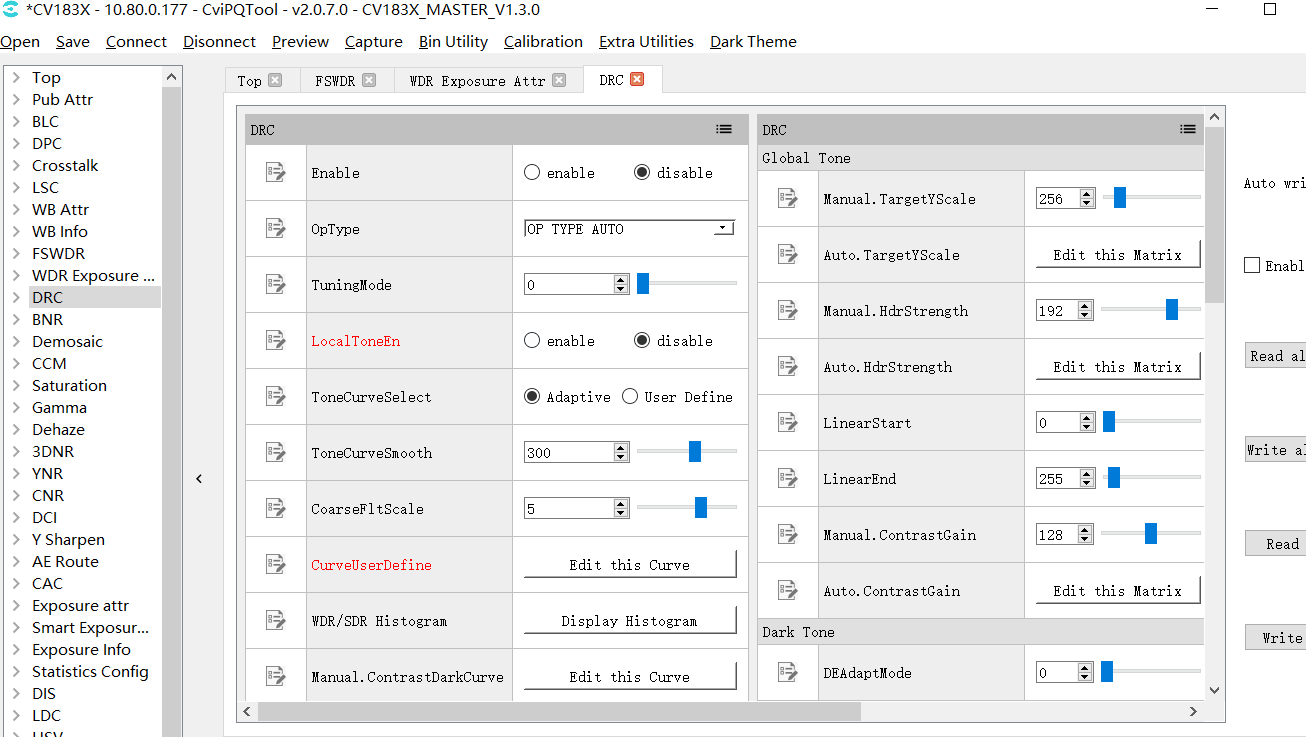
Fig. 3.14 DRC Local-tone switch
3.1.8. 3DNR and YNR Noice Reduction Tuning
The tuning parameters related to noise reduction can be found in 3DNR and YNR pages. For detailed description of noise reduction parameters, please refer to section 3DNR and section YNR in “ISP Tuning Guide”.
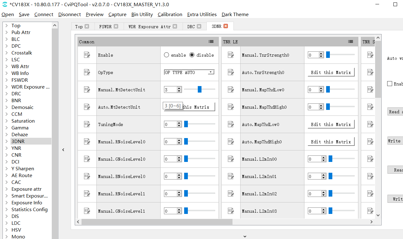
Fig. 3.15 3DNR page
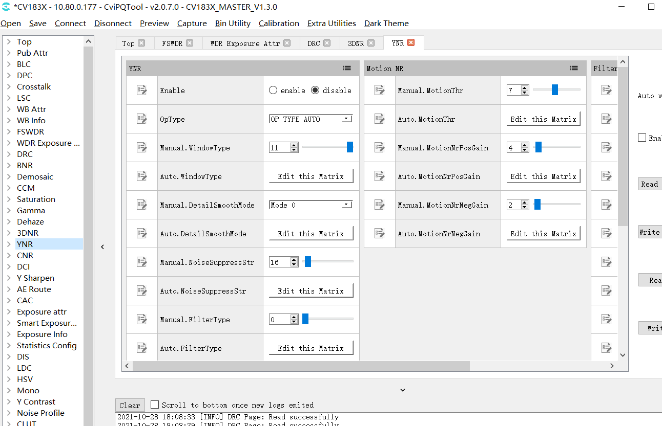
Fig. 3.16 YNR page
3.1.9. Y Sharpen Sharpening and Edge Enhancement Tuning
Y Shapren page contains parameters related to sharpening and edge enhancement. Please refer to section Sharpen of “ISP Tuning Guide” for detailed description of sharpening and edge enhancement parameters.
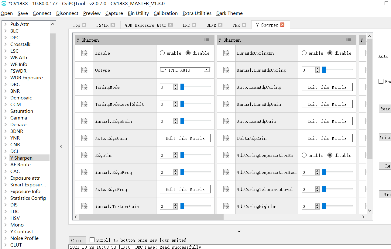
Fig. 3.17 Y Sharpen page
3.1.10. Top Page
The Top page includes ViPipe and ViChn parameters. If there are two sensors on the board end, Vipipe can be used to switch the tuning parameters of different sensors. In addition, Vichn can be used to switch the image of the sensor to be displayed on the screen.
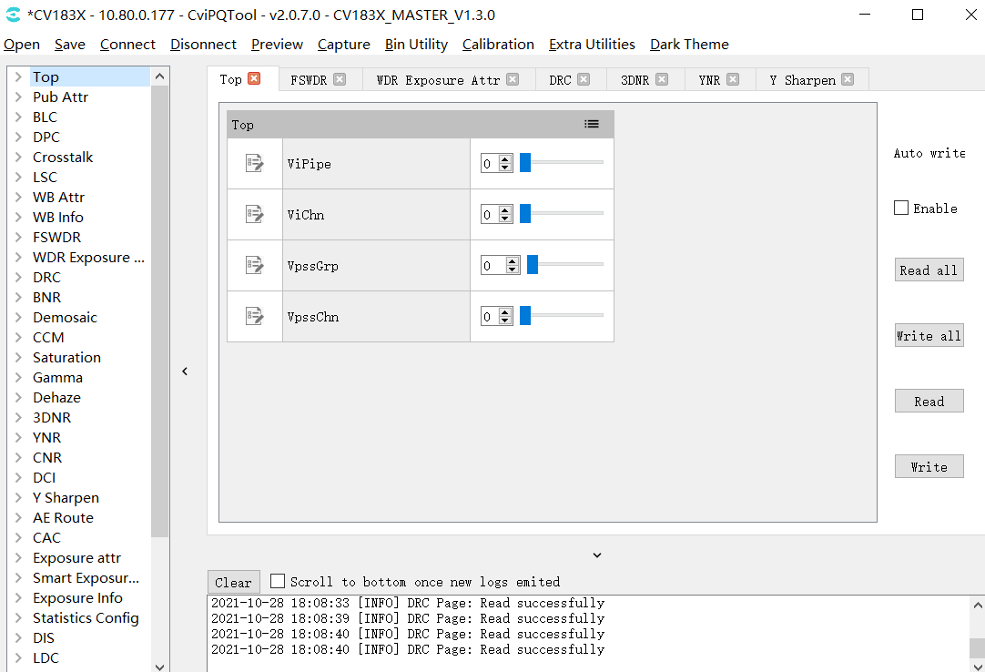
Fig. 3.18 Top page
3.1.11. VPSS Adjustment Page
The VPSS Adustment page is used to tune vpss-related parameters, and the following points should be noted in the tuning process.
During tuning with pqtool, the scene id and vpss grp id are one-to-one, that is, the parameters of scene0 will be written to grp 0;
When App is actually used, it should call CVI_VPSS_SetGrpParamfromBin after each load pq bin to set the binding relationship between scene and vpss grp id, and the vpss parameters in pq bin will take effect at the same time. Otherwise, the vpss parameters tuned with pqtool will not take effect after load pq bin.
Note: the reason for this design is that it is not possible to predict which vpss grp id the app will actually use during tuning of the pq parameters, so the tuning is done one by one, and the mapping relationship needs to be specified according to the actual scenario when the app uses the pq bin generated by tuning.
3.1.12. LDC Page
The LDC page is used for tuning VI and VPSS LDC module related parameters, and the following points should be noted in the usage process:
Read all and Write all do not include read/write operations on the LDC page. Therefore, if the LDC page is set to read or write, a separate operation (click the Read or Write button) must be performed on this page to make it effective.
Currently, the LDC operation is performed at the board end and its computation is large and time consuming. It takes about 2 minutes to complete a computation operation and the PQtool needs to wait in the meantime before the next effective operation can be performed on the PQtool.
3.2. ISP Calibration Tool
Please refer to “ISP Tuning Guide” to complete ISP calibration.
3.3. Advanced Functions
3.3.1. Export and Import of Parameters
The parameters of the tool can be imported and exported in the form of configuration files on the PC side, and the tool can also solidify the parameters to the board side.
Please refer to section 2.4.3.1 Save Tuning Data Files and section 2.4.3.2 Open Tuning Data File for the operation of importing and exporting parameters to configuration file on PC.
To solidify the parameters to the board end, or to export and back up the parameters from the board end to the PC local file, please use the BIN utility tool for operation.
3.3.2. Communication Log
After connecting with the board, all data interaction with the board will be recorded and displayed in the communication log window, as shown in Fig. 3.19 . When interacting with the board, the log contains the following information:
Communication time;
Communication mode and parameters;
Communication contents (such as tuning items currently read or written);
If communication error occurs, error message will be displayed.
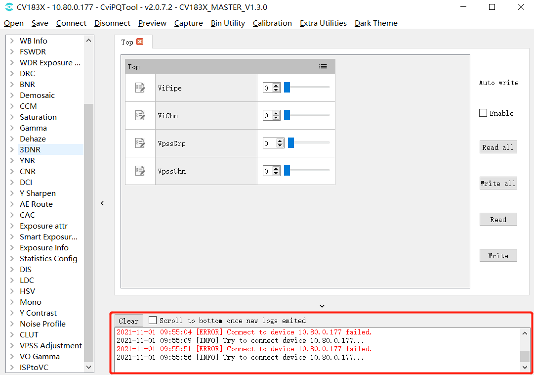
Fig. 3.19 Communiction log window
3.4. Instructions for Other Auxiliary Tools
3.4.1. Instructions for Use of Capture Tool
The image data (YUV and Raw) at the board end can be captured and saved as a local file.
3.4.1.1. Tool Interface
Click the Capture button on the tuning tool menu bar to open the capture tool interface, as shown in Fig. 3.20.
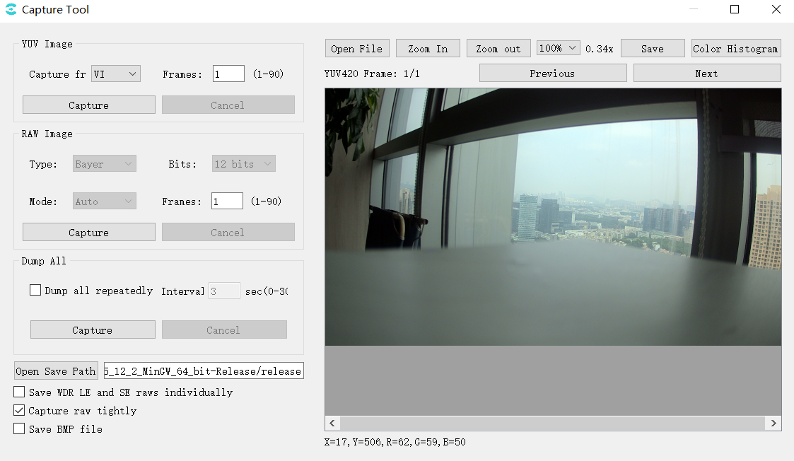
Fig. 3.20 Capture tool interface
Save WDR LE and SE raws individually: when checked, LE raw and SE raw are stored separately; when unchecked, the two raw are stored together.
Capture raw tightly: the way of capturing raw is different, faster when it is checked and slower when it is unchecked.
Save BMP file: when checked a bmp image will be saved, the default is saved in jpg.
At the bottom of the image window, the x,y coordinates and r,g,b values of the point are displayed and change with mouse movement.
Dump all repeatedly: when checked, the dump all will be repeated at the Interval setting time (s).
3.4.1.2. Capture YUV Image Data
Steps to capture YUV data:
In the “YUV image” group box, select the source location of YUV data to capture, that is, select VI / VPSS from the Capture from drop-down menu;
Input the number of frames to capture in the Frames text input box;
Click the Capture button, if the capture is successful, YUV data will be automatically stored in the path position displayed in “Open Save Path”, and YUV data will be displayed in the right image display area, which can be viewed frame by frame by clicking Previous / Next button;
—-Done
3.4.1.3. Capture Raw Image Data
Steps to capture Raw data:
1.Select the bits to capture Raw data in the “Raw Image” group box, that is, select 8bits / 10bits / 12bits / 16bits in the Bits drop-down menu;
2.Select the current mode as Linear, WDR or Auto from the Mode drop-down menu;
3.Input the number of frames to capture in the Frames text input box;
4.Click the “Capture” button, if the capture is successful, Raw and Raw Info data will be automatically stored in the path position displayed in “Open Save Path”, and Raw data will be displayed in the image display area on the right, which can be viewed frame by frame by clicking “Previous / Next” button.
—-Done
3.4.1.4. Dump All
Dump All can capture YUV, RAW images and log information, and capture files as follows:
Capture steps:
1.Set up the yuv capture information in the YUV Image.
2.Set up the raw capture information in the RAW Image.
3.Click the Capture button in Dump All, the tool will first capture and save the raw image and file, then capture and save the yuv image and file, the right image display area will show the raw image, which can be viewed frame by frame by clicking the Previous/Next button.
3.4.1.5. File Name Format Description of YUV Image and RAW Image
The following is the example of file name format of YUV image :

– 1920X1080 means 1920 in width and 1080 in height
– color=3 means BayerID=3 (0: BGGR, 1: GBRG, 2: GRBG, 3: RGGB)
– bits=12 indicates that the significant bits of the image are 12 bits
– frame=1 means that this file contains one YUV image
– 20211101105807 indicates the save time in the format of ”yyyymmddhhmmss”
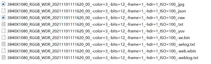
The following is the example of file name of RAW image:

– 3840X1080 means 3840 in width and 1080 in height
– RGGB means ByaerID
– WDR is represented as a wide dynamic image
– color=3 means BayerID=3 (0: BGGR, 1: GBRG, 2: GRBG, 3: RGGB)
– bits=12 indicates that the effective bits of the image are 12 bits
– frame=1 means that this file contains one RAW image
– hdr=1 represents wide dynamic image
– 20211101111620 indicates the save time in the format of ”yyyymmddhhmmss”
The Raw here is decompressed and cropped to: size = width * height * 2 * frame;
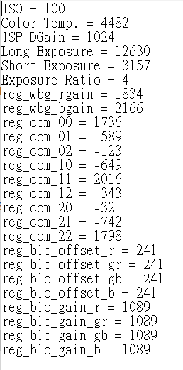
3.4.1.6. File Format and Content Description of Raw Info File
An example of the RAW Info file name format is as follows:

The file name format of RAW Info is exactly the same as that of RAW image, except for the text file with the extension of TXT.
The following is an example of RAW Info file content:
3.4.2. Video Player Instructions (VLC)
3.4.2.1. Steps to use VLC to play video stream on board
Step 1: Download the VLC player. You can download the install-free windows VLC player from the following address : (https://get.videolan.org/vlc/3.0.10/win32/vlc-3.0.10-win32.zip)
For other versions of VLC for other platforms can be downloaded from the VLC website.
Step 2:Open the tool, set VLC parameters, and save and restart VLC.
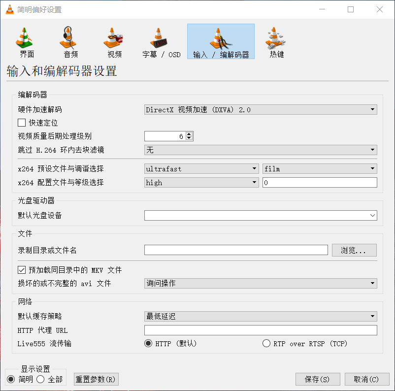
Fig. 3.21 VLC setting interface
Step 3:Use network cable to connect development board and computer. The development board and computer can be directly connected by network cable or connected by router.
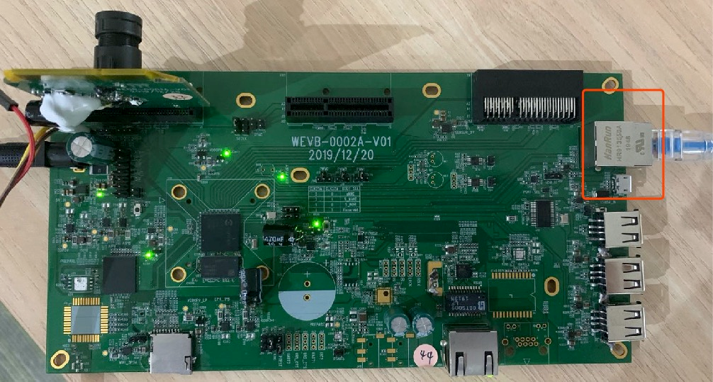
Fig. 3.22 Schematic diagram of network port connection
Step 4:On the board, enter the file system through the serial port and start the CviISPTool program
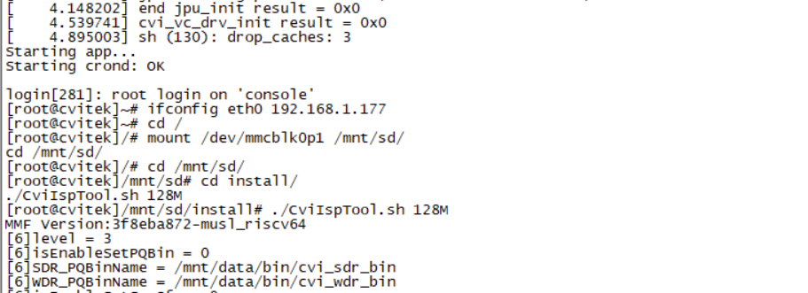
The computer connected with development board needs to be set to the same IP network segment and after mutual ping, VLC can be started to play on the computer connected with development board. The following are some parameters of play setting. After setting, click the play button to see the Sensor screen.
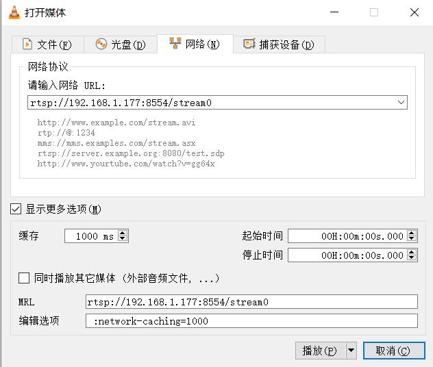
Fig. 3.23 VLC playback parameters setting
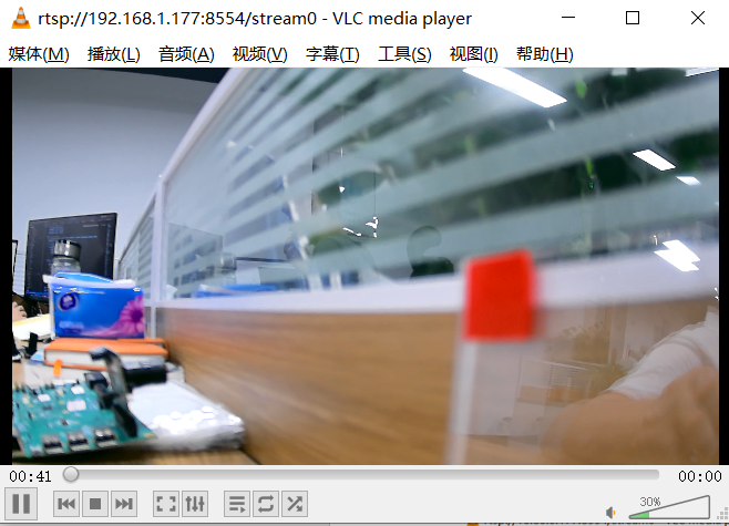
Fig. 3.24 VLC playing video stream
3.4.3. Instructions for Auxiliary Focusing Tool
3.4.3.1. Tool Interface
On the tool home page, select Extra Utilities->Focus Assistant, and the auxiliary focusing interface is shown in the figure below:
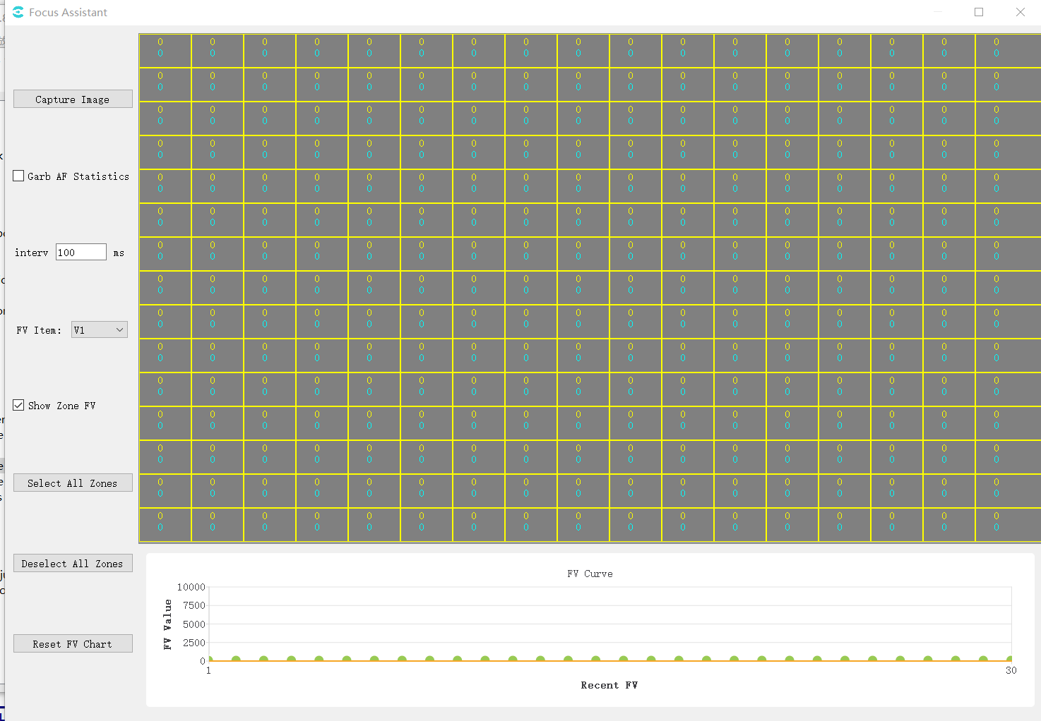
The tool interface is mainly divided into three parts:
(1)Operation area: for various tool operations
(2)Image and interval display area: display the captured image, interval distribution and FV value of each interval (the Yellow value is the current FV value of the interval, and the blue value is the maximum historical FV value of the interval)
(3)FV change curve: display the change curve of global FV value. The point whose abscissa is 1 is the point represented by the nearest FV value. Each time FV value is refreshed, the previous value will be shifted to the right.
3.4.3.2. Use the Auxiliary Focusing Tool to Focus
Steps to focus with the auxiliary focusing tool are as follows:
Step1. Adjust the focal length of the lens to the most blurred state
Step2. Determine the AF interval configuration status of the current device: check grab AF statistics, and remove the check when the number of intervals in the image display area changes.
Step3. Select FV group: select V1 (vertical direction) and H1 (horizontal direction) in FV Item drop-down box.
Step4. Click in the image and interval display area to determine which intervals to focus on. A green circle will be displayed in the upper left corner of the region of interest. You can click “Select All Zones”on the left side of the tool to select all zones, and “Deselect All Zones” to cancel the selection of all zones for easy operation.
Step5. Check “Grab AF Statistics” again. At this time, the image display area and the lower graph begin to refresh continuously.
Step6. Adjust the focal length of the lens. At this time, the blue line of FV curve maximum value increases steadily.
Step7. When observed that the point of position 1 on the FV value curve begins to decline steadily, the position of the maximum blue line should not change (it can be considered that the blue line FV is the theoretical optimal focusing FV). At this time, focus in the opposite direction until the point on position 1 is infinitely close to the blue line position.
3.4.3.3. Focusing Auxiliary Operation
If the user needs to determine which region of the on-demand image belongs to in the focusing process, click “CaptureImage” to capture an image. After the image is displayed in the image area, it can be confirmed.
When “Grab AF statistics” is checked on the tool, the tool will obtain AF statistics from the board end at a fixed time interval. The user can modify the Interval value on the interface to change the interval. The change range is 100-1000 ms.
If the user does not need to view the current value and peak value of FV value between partitions, the show zone FV check box on the left can be unchecked. Remove the check and check again, the interval FV value will be displayed again.
If the user changes the interval configuration, the theoretical FV maximum will change. Users are advised to click the “Reset FV Chart” button at this time. After clicking, the historical global FV value in the lower right chart will be cleared, and the blue line of the maximum FV value will return to zero.
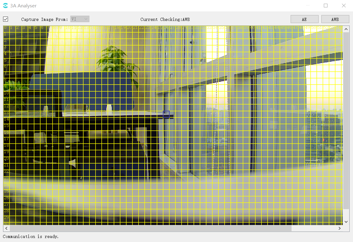
3.4.4. 3A Analyser Tool
3.4.4.1. Tool Interface
In the tool home page, select Extra Utilities -> 3A Analyser in the toolbar, the 3A Analyser interface is as follows:
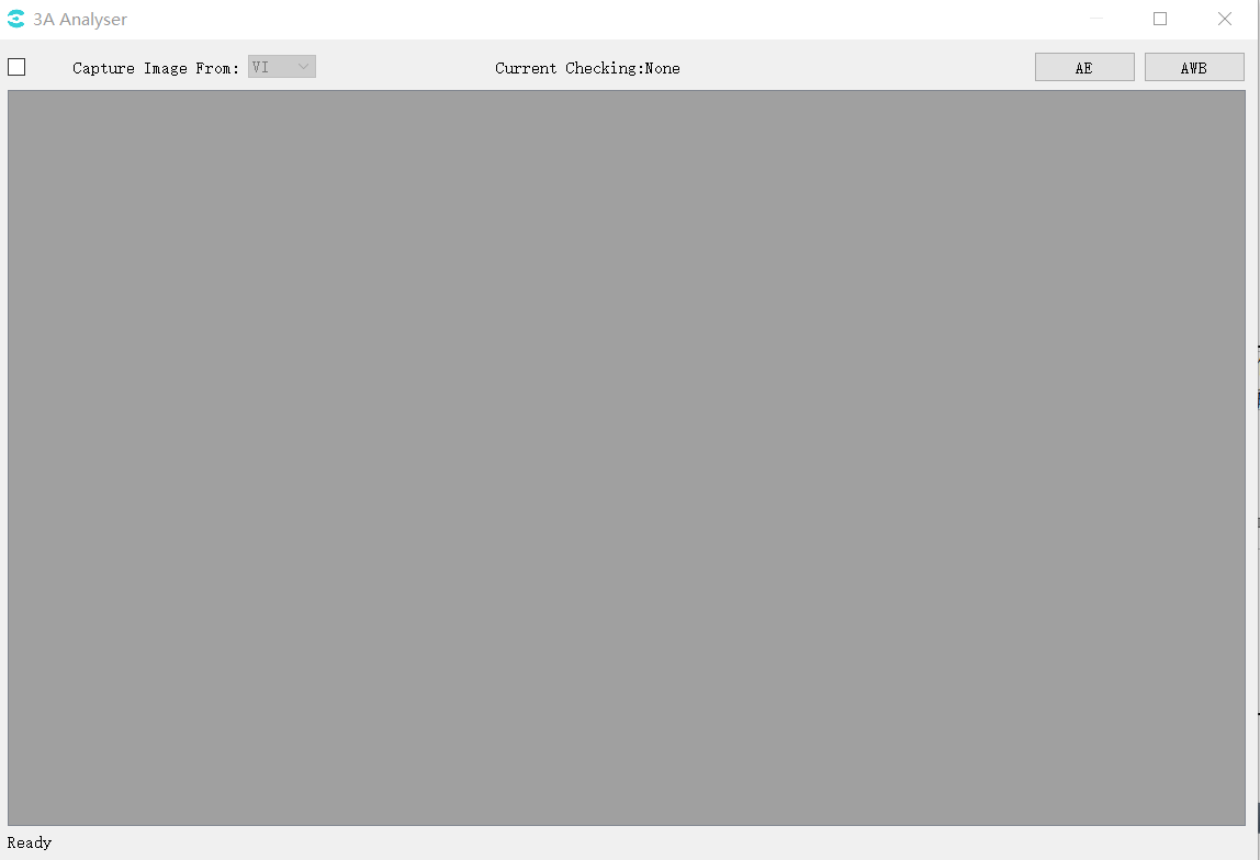
3.4.4.2. Obtain Images and Statistics
CviPQTool connects to the board side.
On the main interface of the 3A Analysis tool, in the drop-down box after Capture Image from, select the image data source (currently the tool only supports acquiring image data from VI).
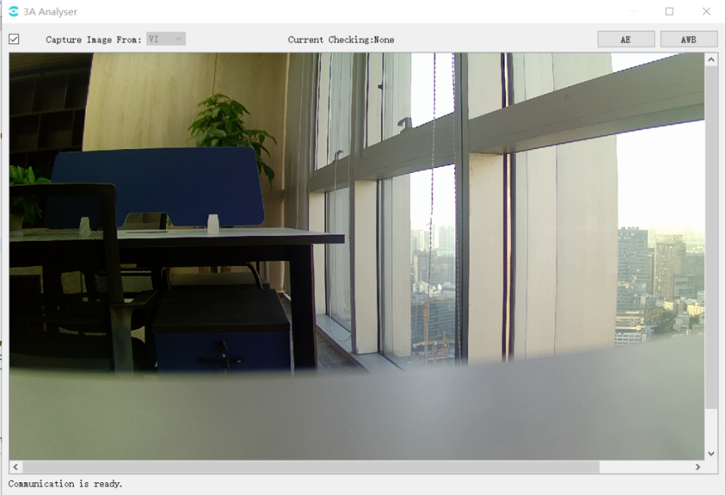
Check the checkbox before Capture Image from. The tool will then automatically capture the data from the board side until the user unchecks the Capture Image from checkbox.
After successfully capturing data from the board side, the tool will display the image effect in the gray area below as shown in the figure below:
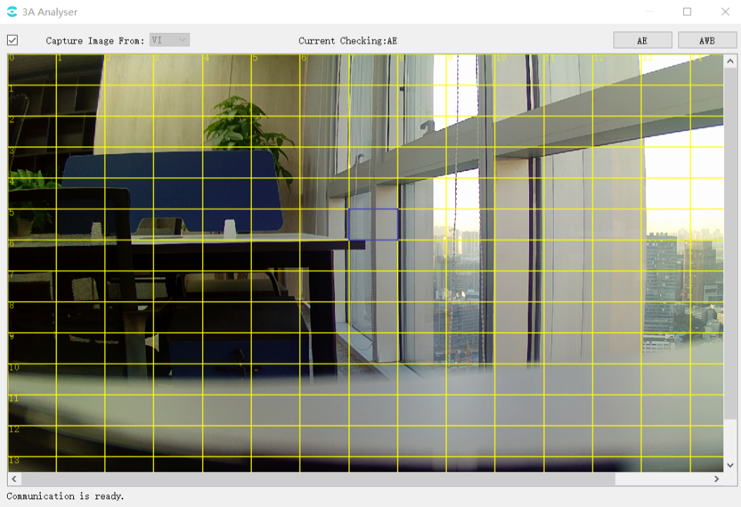
3.4.4.3. View AE Statistics
Click the AE button in the upper right corner of the 3A Analyser tool interface to open the AE statistics window as shown below:
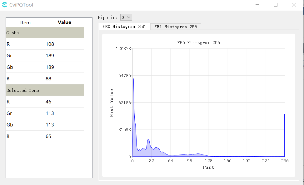
At the same time, the image area of the main interface of 3A Analyser will be divided into intervals by yellow lines, and users can use the mouse The user can use the left mouse button to select the interval, as shown in the figure below.
Statistical information: The average value of the components of Global and Selected Zone can be viewed. When switching the selection zone in the main screen of 3A Analyser, the statistical information data of the selected zone will change.
3.4.4.4. View AWB Statistics
Click the AWB button in the upper right corner of the 3A Analyser interface to open the AWB statistics window as shown below.
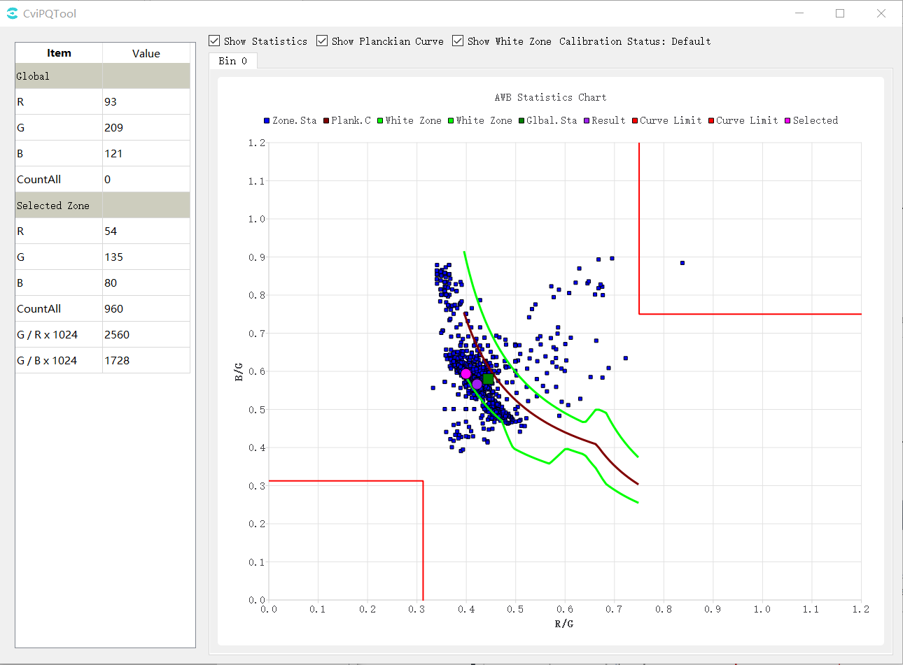
At the same time, the image area of the main interface of 3A Analyser is also divided into intervals by yellow lines. The user can use the left mouse button to select the interval, as shown in the following figure.
The following are shown on the statistical chart.
Red-brown curve: Planck curve (plank.c).
Green point: the point on the Planck coordinate system corresponding to the global statistics.
Purple point: the point corresponding to the result of AWB calculation on the Planck coordinate system.
Blue point: the point on the Planck coordinate system corresponding to the statistical information of the subinterval.
Red point: the point on the Planck coordinate system corresponding to the selected zone of the image selected by the mouse.
Green curve: base white zone interval.
The area enclosed by the red lines at the top right and bottom left: the intervals excluded from the white zone to exclude purple and green interference, respectively, are related to CurveLLimit and CurveRLimit in the AWB parameters.
Show Statistics, ShowPlanckian Curve, and ShowWhite Zone above the image control the display and hiding of statistics, color temperature curves, and white zone intervals on the coordinate map, respectively.
3.4.5. Bracketing
Select Extra Utilities -> Bracketing in the toolbar and the Bracketing window is shown below.
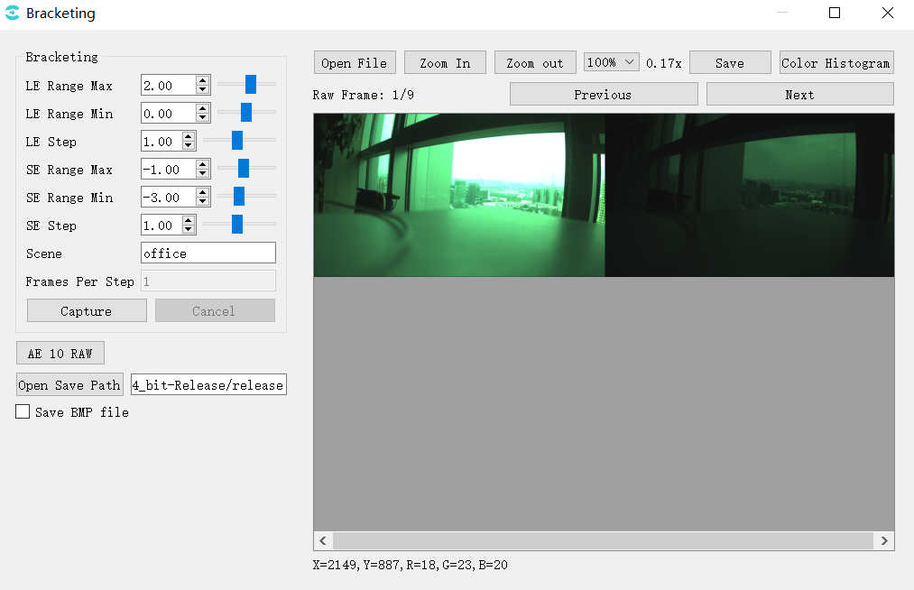
LE/SE Max: Set long and short exposure maximum
LE/SE Min: Set long and short exposure minimum
LE/SE Step: Step length
Capture: Capture the raw of different exposure combinations set by LE/SE
AE 10 RAW: Capture 10 raw of a specific exposure
Save BMP file: Save BMP images, default save as JPG
Open Save Path: File saving directory
Calculation of the number of captured pictures.
LeNum = (LeMax - LeMin) / LeStep + 1;
SeNum = (SeMax - SeMin) / SeStep + 1;
wdr: TotalNum = LeNum * SeNum;
linear: TotalNum = LeNum
3.4.6. Continuous Raw Tool
Select Extra Utilities -> Continuous Raw in the toolbar and the Continuous Raw tool is shown below .
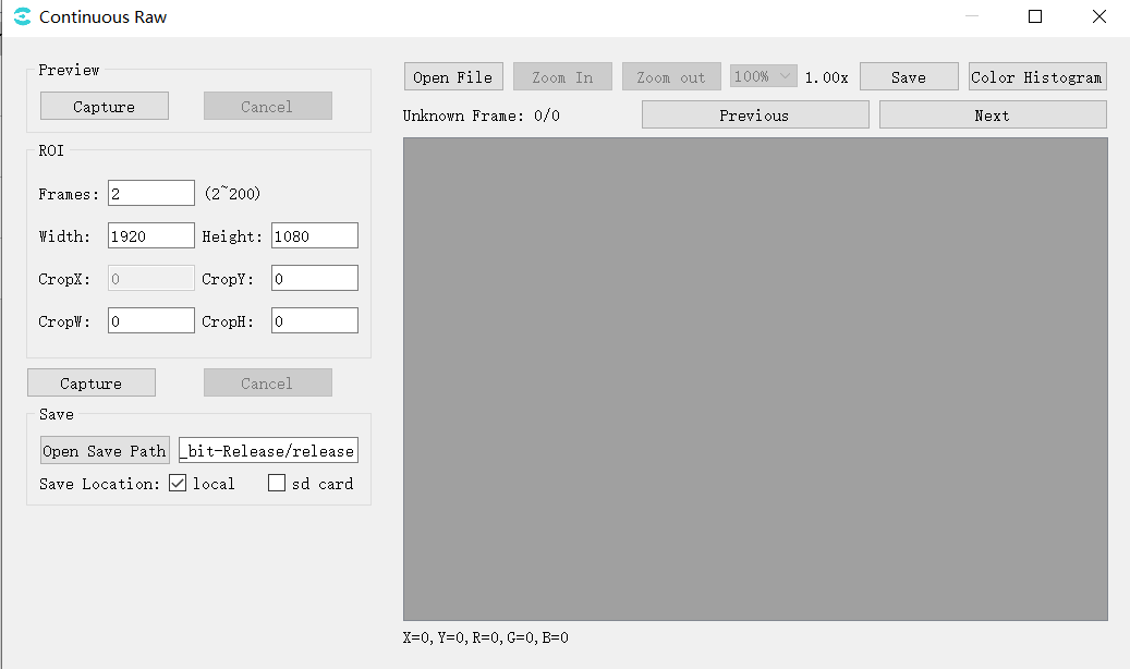
Preview: Preview the current screen
Captur: Click on “capture” to capture the yuv and display it in the right window;
ROI: Capture raw settings
Frames:Capture raw number of frames;
Width/Height:The width and height of the current screen;
CropX/CropY/CropW/CropH:Set the size and position of capturing raw;
Capture:Start capturing raw;
Save: Save settings
Open Save Path:Select the save path;
Save Location:Select save location, select local, raw file will be saved on pc side; select sd card, raw file will be saved on board side;
The capturing files are shown Fig. 3.25 :
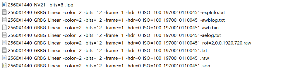
Fig. 3.25 The capturing files
The raw image here is compressed and the size is calculated as follows:
Full size raw
Size = (width * 6 / 8 + 15) / 16 * height * frame;
If Width > 2304, the compression mode is tile, Width needs to be added by 8.
roi raw
Size = (CropW * 6 / 8 + 15) / 16 * CropH * frame;
If Width > 2304, CropW > 1536 and the compression mode is tile,CropW needs to be added by 8.
3.5. Detail Description of Parameters
The following is the description of API function reference of SDK corresponding to each module parameter on the tool interface, as shown in Table 3-2~ Table3-42.
Function Module |
Corresponding SDK API |
|---|---|
Mode Handle |
N/A |
Bypass Setting |
CVI_ISP_SetModuleControl CVI_ISP_GetModuleControl |
Fmw State |
CVI_ISP_SetFMWState CVI_ISP_GetFMWState |
CTRL Param |
CVI_ISP_SetCtrlParam CVI_ISP_GetCtrlParam |
Repeat |
CVI_ISP_SetPipeRepeatMode CVI_ISP_GetPipeRepeatMode |
MOD Param |
CVI_ISP_SetModParam CVI_ISP_GetModParam |
Function Module |
Corresponding SDK API |
|---|---|
PubAttr |
CVI_ISP_SetPubAttr CVI_ISP_GetPubAttr |
Function Module |
Corresponding SDK API |
|---|---|
ISPInfo |
CVI_ISP_QueryInnerStateInfo |
Function Module |
Corresponding SDK API |
|---|---|
ExposureAttr |
CVI_ISP_SetExposureAttr CVI_ISP_GetExposureAttr |
Function Module |
Corresponding SDK API |
|---|---|
WDRExposureAttr |
CVI_ISP_SetWDRExposureAttr CVI_ISP_GetWDRExposureAttr |
Function Module |
Corresponding SDK API |
|---|---|
ExposureInfo |
CVI_ISP_QueryExposureInfo |
Function Module |
Corresponding SDK API |
|---|---|
AERoute |
CVI_ISP_SetAERouteAttr CVI_ISP_GetAERouteAttr CVI_ISP_GetAERouteAttrEx CVI_ISP_SetAERouteAttrEx |
Function Module |
Corresponding SDK API |
|---|---|
White Balance |
CVI_ISP_SetWBAttr CVI_ISP_GetWBAttr |
AWBAttr |
CVI_ISP_SetWBAttr CVI_ISP_GetWBAttr |
MWBAttr |
CVI_ISP_SetWBAttr CVI_ISP_GetWBAttr |
AWB Calibration Data |
CVI_ISP_GetWBCalibration CVI_ISP_SetWBCalibration |
AWBAttrEx |
CVI_ISP_GetAWBAttrEx CVI_ISP_SetAWBAttrEx |
Function Module |
Corresponding SDK API |
|---|---|
WBInfo |
CVI_ISP_QueryWBInfo |
Function Module |
Corresponding SDK API |
|---|---|
CCM |
CVI_ISP_SetCCMAttr CVI_ISP_GetCCMAttr |
ColorToneAttr |
CVI_ISP_GetColorToneAttr CVI_ISP_SetColorToneAttr |
Function Module |
Corresponding SDK API |
|---|---|
CLUT Attr |
CVI_MPI_ISP_SetCLutAttr CVI_MPI_ISP_GetCLutAttr |
Function Module |
Corresponding SDK API |
|---|---|
RadialShading Attr |
CVI_MPI_ISP_SetRadialShadingAttr CVI_MPI_ISP_GetRadialShadingAttr |
RadialShading Gain Lut |
CVI_MPI_ISP_SetRadialShadingGainLutAttr CVI_MPI_ISP_GetRadialShadingGainLutAttr |
Function Module |
Corresponding SDK API |
|---|---|
Demosaic |
CVI_MPI_ISP_SetDemosaicAttr CVI_MPI_ISP_GetDemosaicAttr CVI_MPI_ISP_SetDemosaicDemoireAttr CVI_MPI_ISP_GetDemosaicDemoireAttr CVI_MPI_ISP_SetDemosaicFilterAttr CVI_MPI_ISP_GetDemosaicFilterAttr CVI_MPI_ISP_SetDemosaicEEAttr CVI_MPI_ISP_GetDemosaicEEAttr |
Function Module |
Corresponding SDK API |
|---|---|
AntiFalse |
CVI_ISP_SetAntiFalseColorAttr CVI_ISP_SetAntiFalseColorAttr |
Function Module |
Corresponding SDK API |
|---|---|
3DNR |
CVI_ISP_GetTNRAttr CVI_ISP_SetTNRAttr CVI_ISP_GetTNRNoiseModelAttr CVI_ISP_SetTNRNoiseModelAttr CVI_ISP_GetTNRLumaMotionAttr CVI_ISP_SetTNRLumaMotionAttr CVI_ISP_GetTNRGhostAttr CVI_ISP_SetTNRGhostAttr CVI_ISP_GetTNRMtPrtAttr CVI_ISP_SetTNRMtPrtAttr |
Function Module |
Corresponding SDK API |
|---|---|
DRC |
CVI_ISP_SetDRCAttr CVI_ISP_GetDRCAttr |
Function Module |
Corresponding SDK API |
|---|---|
FSWDR |
CVI_ISP_SetFSWDRAttr CVI_ISP_GetFSWDRAttr |
Function Module |
Corresponding SDK API |
|---|---|
Crosstalk |
CVI_ISP_GetCrosstalkAttr CVI_ISP_SetCrosstalkAttr |
Function Module |
Corresponding SDK API |
|---|---|
Dehaze |
CVI_ISP_SetDehazeAttr CVI_ISP_GetDehazeAttr |
Function Module |
Corresponding SDK API |
|---|---|
Shading Attr |
CVI_ISP_SetMeshShadingAttr CVI_ISP_GetMeshShadingAttr |
Shading Lut Attr |
CVI_ISP_SetMeshShadingGainLutAttr CVI_ISP_GetMeshShadingGainLutAttr |
Function Module |
Corresponding SDK API |
|---|---|
Dynamic Attribute |
CVI_ISP_GetDPDynamicAttr CVI_ISP_SetDPDynamicAttr |
Static Attribute |
CVI_ISP_GetDPStaticAttr CVI_ISP_SetDPStaticAttr |
Function Module |
Corresponding SDK API |
|---|---|
CAC |
CVI_ISP_SetCACAttr CVI_ISP_GetCACAttr |
Function Module |
Corresponding SDK API |
|---|---|
CNR Attr |
CVI_ISP_SetCNRAttr CVI_ISP_GetCNRAttr |
Function Module |
Corresponding SDK API |
|---|---|
DCI |
CVI_ISP_SetDCIAttr CVI_ISP_GetDCIAttr |
Function Module |
Corresponding SDK API |
|---|---|
Gamma |
CVI_ISP_SetGammaAttr CVI_ISP_GetGammaAttr |
Function Module |
Corresponding SDK API |
|---|---|
DRC |
CVI_MPI_ISP_SetDRCAttr CVI_MPI_ISP_GetDRCAttr |
Function Module |
Corresponding SDK API |
|---|---|
FSWDR |
CVI_MPI_ISP_SetFSWDRAttr CVI_MPI_ISP_GetFSWDRAttr |
Function Module |
Corresponding SDK API |
|---|---|
HSV Attr |
CVI_ISP_GetHSVAttr CVI_ISP_SetHSVAttr |
Function Module |
Corresponding SDK API |
|---|---|
LUT 3D |
TBD |
Function Module |
Corresponding SDK API |
|---|---|
YNR |
CVI_ISP_SetYNRAttr CVI_ISP_GetYNRAttr CVI_ISP_SetYNRMotionNRAttr CVI_ISP_GetYNRMotionNRAttr CVI_ISP_SetYNRFilterAttr CVI_ISP_GetYNRFilterAttr |
Function Module |
Corresponding SDK API |
|---|---|
Sharpen |
CVI_ISP_GetSharpenAttr CVI_ISP_SetSharpenAttr |
Function Module |
Corresponding SDK API |
|---|---|
Black Level |
CVI_ISP_GetBlackLevelAttr CVI_ISP_SetBlackLevelAttr |
Function Module |
Corresponding SDK API |
|---|---|
BNR |
CVI_ISP_SetNRAttr CVI_ISP_GetNRAttr |
RLSC |
CVI_ISP_SetRLSCAttr CVI_ISP_GetRLSCAttr |
Filter |
CVI_ISP_SetNRFilterAttr CVI_ISP_GetNRFilterAttr |
Function Module |
Corresponding SDK API |
|---|---|
Saturation |
CVI_ISP_GetSaturationAttr CVI_ISP_SetSaturationAttr |
Function Module |
Corresponding SDK API |
|---|---|
AE/AF/AWB Config |
CVI_ISP_GetStatisticsConfig CVI_ISP_SetStatisticsConfig |
Function Module |
Corresponding SDK API |
|---|---|
DIS Attr |
CVI_ISP_GetDisAttr CVI_ISP_GetDisAttr |
DIS Config |
CVI_ISP_GetDisConfig CVI_ISP_SetDisConfig |
Function Module |
Corresponding SDK API |
|---|---|
VI LDC |
CVI_VI_GetChnLDCAttr CVI_VI_SetChnLDCAttr |
VPSS LDC |
CVI_VPSS_GetChnLDCAttr CVI_VPSS_SetChnLDCAttr |
Function Module |
Corresponding SDK API |
|---|---|
Mono |
CVI_ISP_GetMonoAttr CVI_ISP_SetMonoAttr |
Function Module |
Corresponding SDK API |
|---|---|
YContrast Attr |
CVI_ISP_GetYContrastAttr CVI_ISP_SetYContrastAttr |
Function Module |
Corresponding SDK API |
|---|---|
VPSS Adjustment |
CVI_VPSS_GetGrpProcAmp CVI_VPSS_SetGrpProcAmp |
Function Module |
Corresponding SDK API |
|---|---|
NoiseProfile |
CVI_ISP_GetNoiseProfileAttr CVI_ISP_SetNoiseProfileAttr |