7. Calibration

7.1. General introduction

Calibration is the use of real scene data to tune the proper quantization parameters. Why do we need calibration? When we perform asymmetric quantization of the activation, we need to know the overall dynamic range, i.e., the minmax value, in advance. When applying symmetric quantization to activations, we need to use a suitable quantization threshold algorithm to calculate the quantization threshold based on the overall data distribution of the activation. However, the general trained model does not have the activation statistics. Therefore, both of them need to inference on a miniature sub-training set to collect the output activation of each layer. Then aggregate them to obtain the overall minmax and histogram of the data point distribution. The appropriate symmetric quantization threshold is obtained based on algorithms such as KLD. Finally, the auto-tune algorithm will be enabled to tune the quantization threshold of the input activation of a certain int8 layer by making use of the Euclidean distance between the output activation of int8 and fp32 layers. The above processes are integrated together and executed in unison. The optimized threshold and min/max values for each op are saved in a text file for quantization parameters. Int8 quantization can be achieved by using this text file in model_deploy.py. The overall process is shown in the figure (Overall process of quantization).

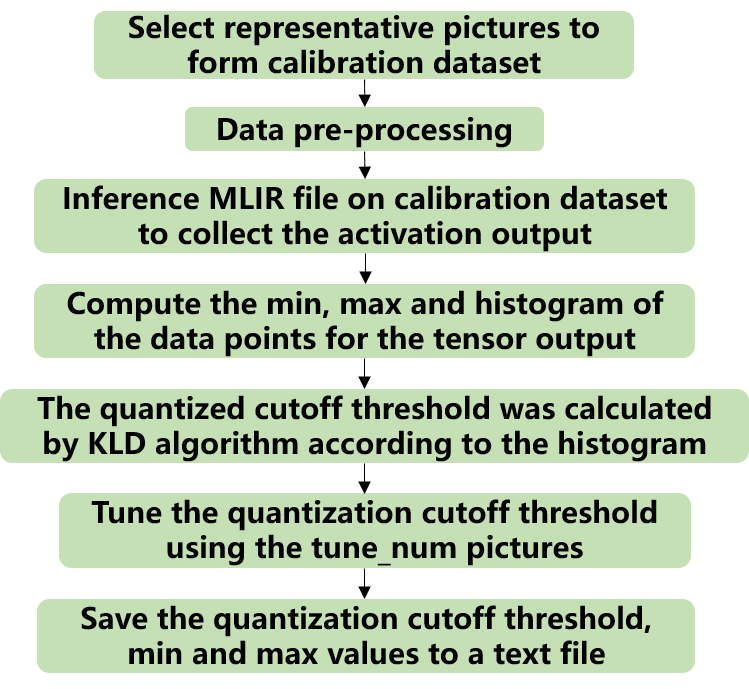
Fig. 7.1 Overall process of quantization

The following figure (Example of quantization parameters file) shows the final output of the calibration quantization parameters file

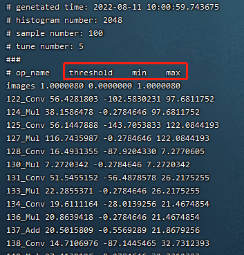
Fig. 7.2 Example of quantization parameters file

7.2. Calibration data screening and preprocessing

7.2.1. Screening Principles

Selecting about 100 to 200 images covering each typical scene style in the training set for calibration. Using a approach similar to training data cleaning to exclude some anomalous samples.

7.2.2. Input format and preprocessing

Table 7.1 Input format

Format	Description
Original Image	For CNN-like vision networks, image input is supported. Image preprocessing arguments must be the same as in training step when generating the mlir file by model_transform.py.
npz or npy file	For cases where non-image inputs or image preprocessing types are not supported at the moment, it is recommended to write an additional script to save the preprocessed input data into npz/npy files (npz file saves multiple tensors in the dictionary, and npy file only contains one tensor). run_calibration.py supports direct input of npz/npy files.

There is no need to specify the preprocessing parameters for the above two formats when calling run_calibration.py to call the mlir file for inference.

Table 7.2 Methods of speciying parameters

Method	Description
–dataset	For single-input networks, place images or preprocessed input npy/npz files (no order required). For multi-input networks, place the pre-processed npz files of each sample.
–data_list	Place the path of the image, npz or npy file of each sample (one sample per line) in a text file. If the network has more than one input file, separate them by commas (note that the npz file should have only 1 input path).

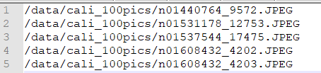
Fig. 7.3 Example of data_list required format

7.3. Algorithm Implementation

7.3.1. KLD Algorithm

The KLD algorithm implemented by tpu-mlir refers to the implementation of tensorRT. In essence, it cuts off some high-order outliers (the intercepted position is fixed at 128 bin, 256bin … until 2048 bin) from the waveform of abs (fp32_tensor) (represented by the histogram of 2048 fp32 bins) to get the fp32 reference probability distribution P. This fp32 waveform is expressed in terms of 128 ranks of int8 type. By merging multiple adjacent bins (e.g., 256 bins are 2 adjacent fp32 bins) into 1 rank of int8 values, calculating the distribution probability, and then expanding bins to ensure the same length as P, the probability distribution Q of the quantized int8 values can be got. The KL divergences of P and Q are calculated for the interception positions of 128bin, 256bin, …, and 2048 bin, respectively in each loop until the interception with the smallest divergence is found. Interception here means the probability distribution of fp32 can be best simulated with the 128 quantization levels of int8. Therefore, it is most appropriate to set the quantization threshold here. The pseudo-code for the implementation of the KLD algorithm is shown below:

the pseudocode of computing int8 quantize threshold by kld:
    Prepare fp32 histogram H with 2048 bins
    compute the absmax of fp32 value

    for i in range(128,2048,128):
      Outliers_num=sum(bin[i], bin[i+1],…, bin[2047])
      Fp32_distribution=[bin[0], bin[1],…, bin[i-1]+Outliers_num]
      Fp32_distribution/= sum(Fp32_distribution)

      int8_distribution = quantize [bin[0], bin[1],…, bin[i]] into 128 quant level
      expand int8_distribution to i bins
      int8_distribution /= sum(int8_distribution)
      kld[i] = KLD(Fp32_distribution, int8_distribution)
    end for

    find i which kld[i] is minimal
    int8 quantize threshold = (i + 0.5)*fp32 absmax/2048

7.3.2. Auto-tune Algorithm

From the actual performance of the KLD algorithm, its candidate threshold is relatively coarse and does not take into account the characteristics of different scenarios, such as object detection and key point detection, in which tensor outliers may be more important to the performance. In these cases, a larger quantization threshold is required to avoid saturation which will affect the expression of distribution features. In addition, the KLD algorithm calculates the quantization threshold based on the similarity between the quantized int8 and the fp32 probability distribution, while there are other methods to evaluate the waveform similarity such as Euclidean distance, cos similarity, etc. These metrics evaluate the tensor numerical distribution similarity directly without the need for a coarse interception threshold, which most of the time has better performance. Therefore, with the basis of efficient KLD quantization threshold, tpu-mlir proposes the auto-tune algorithm to fine-tune these activations quantization thresholds based on Euclidean distance metric, which ensures a better accuracy performance of its int8 quantization.

Implementation: firstly, uniformly pseudo-quantize layers with weights in the network, i.e., quantize their weights from fp32 to int8, and then de-quantize to fp32 for introducing quantization error. After that, tune the input activation quantization threshold of op one by one (i.e., uniformly select 10 candidates among the initial KLD quantization threshold and maximum absolute values of activations. Use these candidates to quantize fp32 reference activation values for introducing quantization error. Input op for fp32 calculation, calculating the Euclidean distance between the output and the fp32 reference activations. The candidate with a minimum Euclidean distance will be selected as the tuning threshold). For the case where the output of one op is connected to multiple subsequent ones, the quantization thresholds are calculated for the multiple branches according to the above method, and then the larger one is taken. For instance, the output of layer1 will be adjusted for layer2 and layer3 respectively as shown in the figure (Implementation of auto-tune).

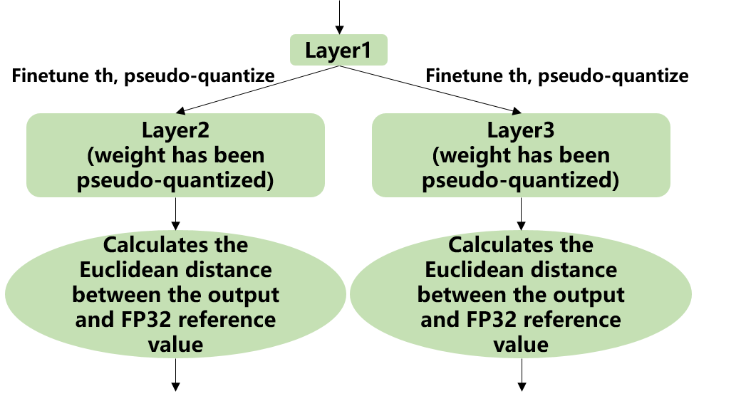
Fig. 7.4 Implementation of auto-tune

7.4. Example: yolov5s calibration

In the docker environment of tpu-mlir, execute source envsetup.sh in the tpu-mlir directory to initialize the environment, then enter any new directory and execute the following command to complete the calibration process for yolov5s.

$ model_transform.py \
   --model_name yolov5s \
   --model_def  ${REGRESSION_PATH}/model/yolov5s.onnx \
   --input_shapes [[1,3,640,640]] \
   --keep_aspect_ratio \  #keep_aspect_ratio、mean、scale、pixel_format are preprocessing arguments
   --mean 0.0,0.0,0.0 \
   --scale 0.0039216,0.0039216,0.0039216 \
   --pixel_format rgb \
   --output_names 350,498,646 \
   --test_input ${REGRESSION_PATH}/image/dog.jpg \
   --test_result yolov5s_top_outputs.npz \
   --mlir yolov5s.mlir

$ run_calibration.py yolov5s.mlir \
   --dataset $REGRESSION_PATH/dataset/COCO2017 \
   --input_num 100 \
   --tune_num 10 \
   -o yolov5s_cali_table

The result is shown in the following figure (yolov5s_cali calibration result).

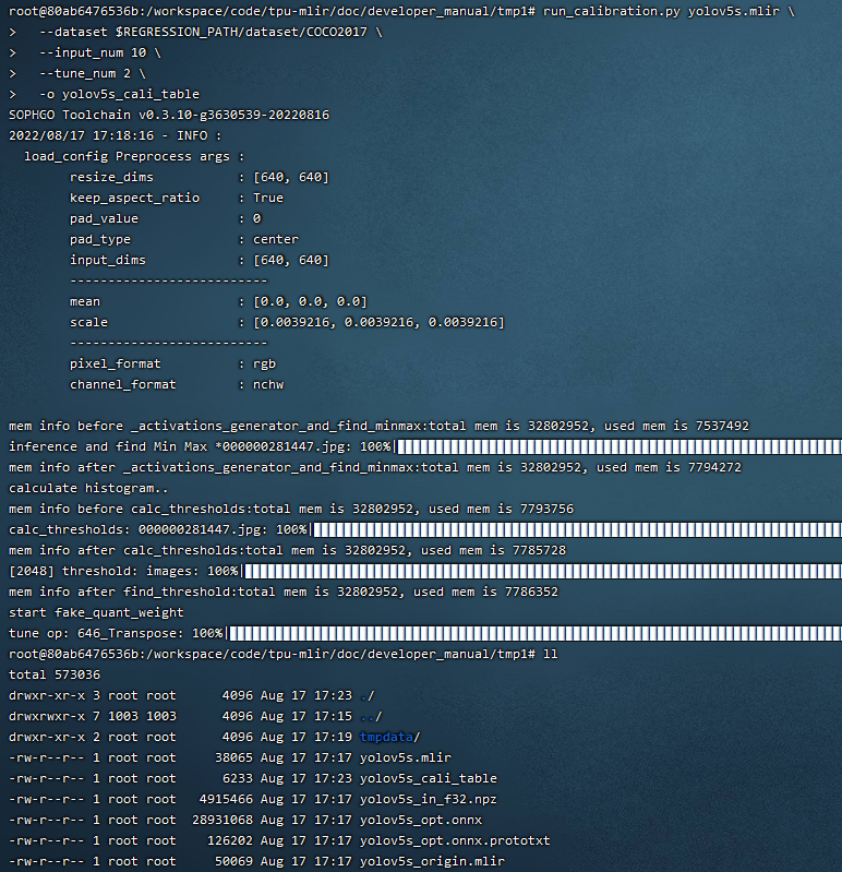
Fig. 7.5 yolov5s_cali calibration result

7.5. visual tool introduction

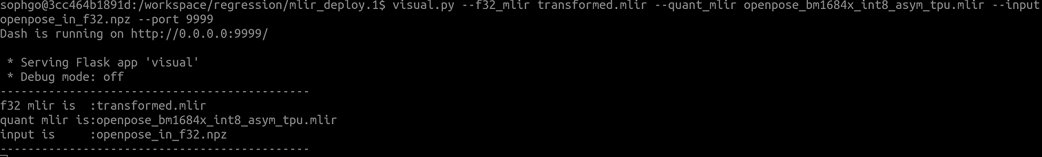
visual.py is an visualized net/tensor compare tool with UI in web browser. When quantized net encounters great accuracy decrease, this tool can be used to investigate the accuracy loss layer by layer. This tool is started in docker as an server listening to TCP port 10000 (default), and by input localhost:10000 in url of browser in host computer, the tool UI will be displayed in it, the port must be mapped to host in advance when starting the docker, and the tool must be start in the same directory where the mlir files located, start command is as following:

Table 7.3 visual tool parameters

Param	Description
–port	the TCP port used to listen to browser as server, default value is 10000
–f32_mlir	the float mlir net to compare to
–quant_mlir	the quantized mlir net to compare with float net
–input	input data to run the float net and quantized net for data compare, can be image or npy/npz file, can be the test_input when graph_transform
–manual_run	if run the nets when browser connected to server, default is true, if set false, only the net structure will be displayed

Open browser in host computer and input localhost:9999, the tool UI will be displayed. The float and quantized net will automatically inference to get output of every layer, if the nets are huge, it would took a long time to wait! UI is as following:

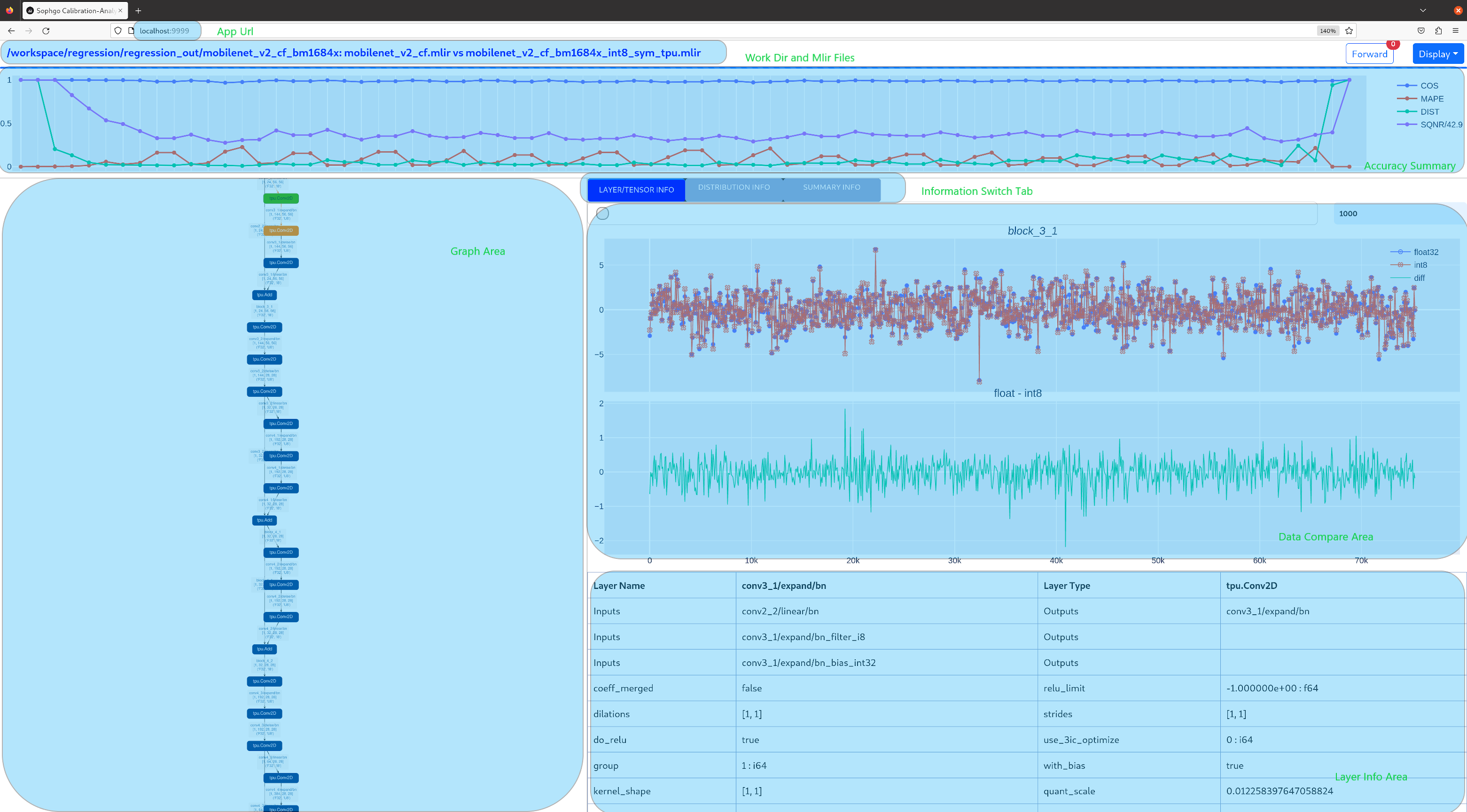
Areas of the UI is marked with light blue rectangle for reference, dark green comments on the areas, includeing:

1. working directory and net file indication

2. accuracy summary area

3. layer information area

4. graph display area

5. tensor data compare figure area

6. infomation summary and tensor distribution area (by switching tabs)

With scroll wheel over graph display area, the displayed net graph can be zoomed in and out, and hover or click on the nodes (layer), the attributes of it will be displayed in the layer information card, by clicking on the edges (tensor), the compare of tensor data in float and quantized net is displayed in tensor data compare figure, and by clicking on the dot in accuracy summary or information list cells, the layer/tensor will be located in graph display area.

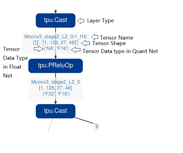
Notice: the net graph is displayed according to quantized net, and there may be difference in it comparing to float net, some layer/tensor may not exist in float net, but the data is copied from quantized net for compare, so the accuracy may seem perfect, but in fact, it should be ignored. Typical layer is Cast layer in quantized net, in following picture, the non-exist tensor data type will be NA. Notice: without –debug parameter in deployment of the net, some essential intermediate files needed by visual tool would have been deleted by default, please re-deploy with –debug parameter.

information displayed on edge (tensor) is illustrated as following: